卷积神经网络
Table of Contents
import tensorflow as tf
import numpy as np
import matplotlib.pyplot as plt
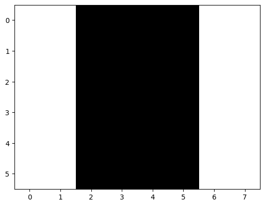
# 1. 构造一个简单的图像
X = np.ones((6, 8))
X[:, 2:6] = 0
print(X.shape)
plt.imshow(X, cmap='gray')
plt.show()
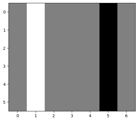
K = np.array([[1.0, -1.0]])
# 输入图像转换格式为 [batch, height, width, channels]
# 卷积核转换格式为 [filter_height, filter_width, in_channels, out_channels]
Y = tf.nn.conv2d(X.reshape((1, 6, 8, 1)), K.reshape((1, 2, 1, 1)), strides=[1, 1, 1, 1], padding='VALID')
print(Y.shape)
plt.imshow(Y.numpy().reshape(6,7), cmap='gray')
plt.show()
#将两幅图像对比绘制
# 创建一个画布,其中包含两个子图,布局为2行1列
fig, axs = plt.subplots(2, 1, sharex=True, figsize=(10, 8)) # figsize的单位是英寸
# 绘制第一张图
axs[0].imshow(X, cmap='gray')
axs[0].set_title('X')
# 绘制第二张图
axs[1].imshow(Y.numpy().reshape(6,7), cmap='gray')
axs[1].set_title('Y')
# 显示图形
plt.show()
# 加入池化层
max_pool_2d = tf.keras.layers.MaxPooling2D(padding="same")
P=max_pool_2d(Y)
plt.imshow(P.numpy().reshape(3,4), cmap='gray')
plt.show()
# 创建一个画布,其中包含三个子图,布局为3行1列
fig, axs = plt.subplots(3, 1, sharex=True, figsize=(10, 8)) # figsize的单位是英寸
# 绘制第一张图
axs[0].imshow(X, cmap='gray')
axs[0].set_title('X')
# 绘制第二张图
axs[1].imshow(Y.numpy().reshape(6,7), cmap='gray')
axs[1].set_title('Y')
# 绘制第三张图
axs[2].imshow(P.numpy().reshape(3,4), cmap='gray')
axs[2].set_title('P')
# 显示图形
plt.show()
import torch
import torch.nn as nn
import numpy as np
import matplotlib.pyplot as plt
from PIL import Image
import torchvision.transforms.functional as TF

# 1. 加载图像并转为灰度(方便单通道展示)
img = Image.open('D:\\work\\mygithub\\docs\\intoAI\\src\\chapter2\\images\\intoAI_2_1.png').convert('L')
img_tensor = TF.to_tensor(img).unsqueeze(0) # 形状变为 [1, 1, H, W]

# 2. 定义边缘检测卷积核
# 这是一个经典的 Sobel 边缘检测算子
sobel_kernel = torch.tensor([[[-1., -1., -1.],
                              [-1.,  8., -1.],
                              [-1., -1., -1.]]])

# 调整形状为 [1, 1, 3, 3] (输出通道, 输入通道, 卷积核高, 卷积核宽)
kernel = sobel_kernel.view(1, 1, 3, 3)

# 3. 进行卷积操作
# padding=1 保持图像边缘信息,stride=1 逐像素滑动
conv_output = nn.functional.conv2d(img_tensor, kernel, padding=1)

# 4. 可视化
plt.imshow(conv_output.squeeze().numpy(), cmap='gray')
plt.title("Convolution Output (Edge Detection)")
plt.show()


# 1. 对卷积后的特征图进行最大池化 (池化核大小为 2x2,步长为 2)
# 这会让图像的宽和高各缩小一半
max_pool_output = nn.functional.max_pool2d(conv_output, kernel_size=2, stride=2)

# 2. 打印形状对比
print(f"卷积后特征图形状: {conv_output.shape}")
print(f"池化后特征图形状: {max_pool_output.shape}")

# 3. 可视化
plt.imshow(max_pool_output.squeeze().numpy(), cmap='gray')
plt.title("Max Pooling Output (Downsampled)")
plt.show()
max_pool_2d = tf.keras.layers.MaxPooling2D(padding="same")

x = np.array([[1., 2., 3.],
              [4., 5., 6.],
              [7., 8., 9.]])
x = np.reshape(x, [1, 3, 3, 1])
max_pool_2d(x)
import tensorflow as tf
import numpy as np
import matplotlib.pyplot as plt

# 1. 加载图像并转为灰度 --> [batch, height, width, channels]
imagePath = "D:\\work\\mygithub\\docs\\intoAI\\src\\chapter2\\images\\intoAI_2_1.png"
img = tf.keras.utils.load_img(imagePath, color_mode='grayscale')
plt.imshow(img, cmap='gray')
plt.show()
X = np.array(img, dtype='int32' ).reshape(1, 28, 28, 1)

# 2. 定义边缘检测卷积核 --> [filter_height, filter_width, in_channels, out_channels]
# 这是一个经典的 Sobel 边缘检测算子
sobel_kernel = np.array([[[-1., -1., -1.],
                              [-1.,  8., -1.],
                              [-1., -1., -1.]]])
K = sobel_kernel.reshape((3, 3, 1, 1))

# 3. 进行卷积操作
Y = tf.nn.conv2d(X, K, strides=[1, 1, 1, 1], padding='VALID')
print(Y.shape)
plt.imshow(Y.numpy().reshape(26,26), cmap='gray')
plt.show()


# 4. 对卷积后的特征图进行最大池化 (池化核大小为 2x2,步长为 2)
max_pool_2d = tf.keras.layers.MaxPooling2D(pool_size=(2, 2),strides=(1, 1), padding="valid")
max_pool_output = max_pool_2d(Y)

# 5. 打印形状对比
print(f"卷积后特征图形状: {Y.shape}")
print(f"池化后特征图形状: {max_pool_output.shape}")

plt.imshow(max_pool_output.numpy().reshape(25,25), cmap='gray')
plt.show()


import tensorflow as tf
from tensorflow.keras import layers
from tensorflow.keras.models import Sequential
import numpy as np
import matplotlib.pyplot as plt

mnist = tf.keras.datasets.mnist
(x_train, y_train), _ = mnist.load_data()
x_train=x_train.reshape(x_train.shape[0], x_train.shape[1], x_train.shape[2], 1)

batch_size = 64
num_classes = 10
epochs = 10
img_height = 28
img_width = 28

model = Sequential([
  layers.Rescaling(1./255, input_shape=(img_height, img_width, 1)),
  layers.Conv2D(16, 3, padding='same', activation='relu'),
  layers.MaxPooling2D(),
  layers.Conv2D(32, 3, padding='same', activation='relu'),
  layers.MaxPooling2D(),
  layers.Conv2D(64, 3, padding='same', activation='relu'),
  layers.MaxPooling2D(),
  layers.Dropout(0.2),
  layers.Flatten(),
  layers.Dense(128, activation='relu'),
  layers.Dense(num_classes, name="outputs")
])

model.compile(optimizer='adam',
              loss=tf.keras.losses.SparseCategoricalCrossentropy(from_logits=True),
              metrics=['accuracy'])

model.summary()

log_dir = "D:\\mnist\\logs"
tensorboard_callback = tf.keras.callbacks.TensorBoard(log_dir=log_dir, histogram_freq=1)

history = model.fit(
  x_train, y_train,
  batch_size=batch_size,
  validation_split=0.2,
  epochs=epochs,
  callbacks=[tensorboard_callback]
)

acc = history.history['accuracy']
val_acc = history.history['val_accuracy']

loss = history.history['loss']
val_loss = history.history['val_loss']

epochs_range = range(epochs)

plt.figure(figsize=(8, 8))
plt.subplot(1, 2, 1)
plt.plot(epochs_range, acc, label='Training Accuracy')
plt.plot(epochs_range, val_acc, label='Validation Accuracy')
plt.legend(loc='lower right')
plt.title('Training and Validation Accuracy')

plt.subplot(1, 2, 2)
plt.plot(epochs_range, loss, label='Training Loss')
plt.plot(epochs_range, val_loss, label='Validation Loss')
plt.legend(loc='upper right')
plt.title('Training and Validation Loss')
plt.show()

imagePath = "D:\\work\\mygithub\\docs\\intoAI\\src\\chapter2\\images\\intoAI_2_10.bmp"
img = tf.keras.utils.load_img(imagePath, color_mode='grayscale')
print(img.size)  # 输出图像尺寸
print(img.mode)  # 输出图像模式,应为 'L' 表示灰度图像
img_array = (np.expand_dims(img,0))
print(img_array.shape)
predictions = model.predict(img_array)
print(predictions)
score = tf.nn.softmax(predictions[0])
print(np.argmax(score))
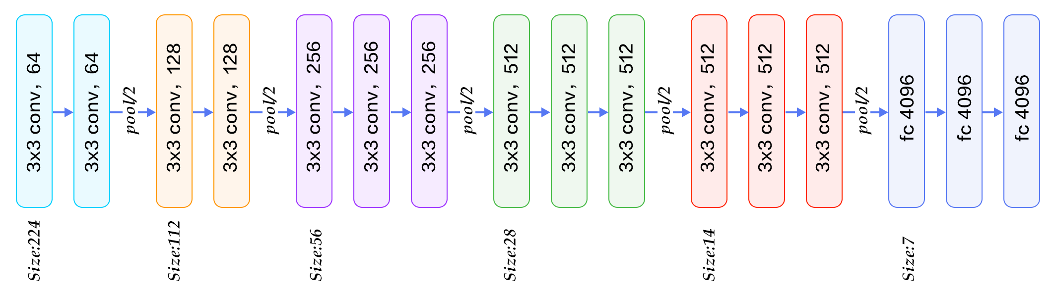
论文:Very Deep Convolutional Networks for Large-Scale Image Recognition
牛津大学VGG研究组:Visual Geometry Group
- VGGNet的结构非常简洁,整个网络都使用了同样大小的卷积核尺寸(3x3)和最大池化尺寸(2x2)
- 几个小滤波器(3x3)卷积层的组合比一个大滤波器(5x5或7x7)卷积层好
- 验证了通过不断加深网络结构可以提升性能
conv1  = Conv2D(filters=64, kernel_size=(3,3), padding="same", activation="relu")(_input)
conv2  = Conv2D(filters=64, kernel_size=(3,3), padding="same", activation="relu")(conv1)
pool1  = MaxPooling2D((2, 2))(conv2)

conv3  = Conv2D(filters=128, kernel_size=(3,3), padding="same", activation="relu")(pool1)
conv4  = Conv2D(filters=128, kernel_size=(3,3), padding="same", activation="relu")(conv3)
pool2  = MaxPooling2D((2, 2))(conv4)

conv5  = Conv2D(filters=256, kernel_size=(3,3), padding="same", activation="relu")(pool2)
conv6  = Conv2D(filters=256, kernel_size=(3,3), padding="same", activation="relu")(conv5)
conv7  = Conv2D(filters=256, kernel_size=(3,3), padding="same", activation="relu")(conv6)
pool3  = MaxPooling2D((2, 2))(conv7)

conv8  = Conv2D(filters=512, kernel_size=(3,3), padding="same", activation="relu")(pool3)
conv9  = Conv2D(filters=512, kernel_size=(3,3), padding="same", activation="relu")(conv8)
conv10 = Conv2D(filters=512, kernel_size=(3,3), padding="same", activation="relu")(conv9)
pool4  = MaxPooling2D((2, 2))(conv10)

conv11 = Conv2D(filters=512, kernel_size=(3,3), padding="same", activation="relu")(pool4)
conv12 = Conv2D(filters=512, kernel_size=(3,3), padding="same", activation="relu")(conv11)
conv13 = Conv2D(filters=512, kernel_size=(3,3), padding="same", activation="relu")(conv12)
pool5  = MaxPooling2D((2, 2))(conv13)

flat   = Flatten()(pool5)
dense1 = Dense(4096, activation="relu")(flat)
dense2 = Dense(4096, activation="relu")(dense1)
output = Dense(1000, activation="softmax")(dense2)

vgg16_model  = Model(inputs=_input, outputs=output)
tiny-vgg:CNN-explainer
import tensorflow as tf
import numpy as np
import pandas as pd
import re
from shutil import copyfile
from glob import glob
from json import load, dump
from tensorflow.keras.layers import Dense, Flatten, Conv2D, MaxPool2D,Activation
from tensorflow.keras import Model, Sequential
from os.path import basename
from time import time
import os

# 数据存放的位置
os.chdir('C:\\Users\\haiye\\Desktop\\data')
print(os.getcwd())


def process_path_train(path):
    """
    Get the (class label, processed image) pair of the given image path. This
    funciton uses python primitives, so you need to use tf.py_funciton wrapper.
    This function uses global variables:

        WIDTH(int): the width of the targeting image
        HEIGHT(int): the height of the targeting iamge
        NUM_CLASS(int): number of classes

    Args:
        path(string): path to an image file
    """

    # Get the class
    path = path.numpy()
    image_name = basename(path.decode('ascii'))
    label_name = re.sub(r'(.+)_\d+\.JPEG', r'\1', image_name)
    label_index = tiny_class_dict[label_name]['index']

    # Convert label to one-hot encoding
    label = tf.one_hot(indices=[label_index], depth=NUM_CLASS)
    label = tf.reshape(label, [NUM_CLASS])

    # Read image and convert the image to [0, 1] range 3d tensor
    img = tf.io.read_file(path)
    img = tf.image.decode_jpeg(img, channels=3)
    img = tf.image.convert_image_dtype(img, tf.float32)
    img = tf.image.resize(img, [WIDTH, HEIGHT])

    return(img, label)


def process_path_test(path):
    """
    Get the (class label, processed image) pair of the given image path. This
    funciton uses python primitives, so you need to use tf.py_funciton wrapper.
    This function uses global variables:

        WIDTH(int): the width of the targeting image
        HEIGHT(int): the height of the targeting iamge
        NUM_CLASS(int): number of classes

    The filepath encoding for test images is different from training images.

    Args:
        path(string): path to an image file
    """

    # Get the class
    path = path.numpy()
    image_name = basename(path.decode('ascii'))
    label_index = tiny_val_class_dict[image_name]['index']

    # Convert label to one-hot encoding
    label = tf.one_hot(indices=[label_index], depth=NUM_CLASS)
    label = tf.reshape(label, [NUM_CLASS])

    # Read image and convert the image to [0, 1] range 3d tensor
    img = tf.io.read_file(path)
    img = tf.image.decode_jpeg(img, channels=3)
    img = tf.image.convert_image_dtype(img, tf.float32)
    img = tf.image.resize(img, [WIDTH, HEIGHT])

    return(img, label)


def prepare_for_training(dataset, batch_size=32, cache=True,
                         shuffle_buffer_size=1000):

    if cache:
        if isinstance(cache, str):
            dataset = dataset.cache(cache)
        else:
            dataset = dataset.cache()

    # Only shuffle elements in the buffer size
    dataset = dataset.shuffle(buffer_size=shuffle_buffer_size)

    # Pre featch batches in the background
    dataset = dataset.batch(batch_size)
    dataset = dataset.prefetch(buffer_size=tf.data.experimental.AUTOTUNE)

    return dataset


@tf.function
def train_step(image_batch, label_batch):
    with tf.GradientTape() as tape:
        # Predict
        predictions = tiny_vgg(image_batch)

        # Update gradient
        loss = loss_object(label_batch, predictions)
        gradients = tape.gradient(loss, tiny_vgg.trainable_variables)
        optimizer.apply_gradients(zip(gradients, tiny_vgg.trainable_variables))

        train_mean_loss(loss)
        train_accuracy(label_batch, predictions)


@tf.function
def vali_step(image_batch, label_batch):
    predictions = tiny_vgg(image_batch)
    vali_loss = loss_object(label_batch, predictions)

    vali_mean_loss(vali_loss)
    vali_accuracy(label_batch, predictions)


@tf.function
def test_step(image_batch, label_batch):
    predictions = tiny_vgg(image_batch)
    test_loss = loss_object(label_batch, predictions)

    test_mean_loss(test_loss)
    test_accuracy(label_batch, predictions)


WIDTH = 64
HEIGHT = 64
EPOCHS = 1000
PATIENCE = 50
LR = 0.001
NUM_CLASS = 10
BATCH_SIZE = 32


# Create training and validation dataset
tiny_class_dict = load(open('./data/class_dict_10.json', 'r'))
tiny_val_class_dict = load(open('./data/val_class_dict_10.json', 'r'))

training_images = './data/class_10_train/*/images/*.JPEG'
vali_images = './data/class_10_val/val_images/*.JPEG'
test_images = './data/class_10_val/test_images/*.JPEG'

# Create training dataset
train_path_dataset = tf.data.Dataset.list_files(training_images)

train_labeld_dataset = train_path_dataset.map(
    lambda path: tf.py_function(
        process_path_train,
        [path],
        [tf.float32, tf.float32]
    )
)


# Create vali dataset
vali_path_dataset = tf.data.Dataset.list_files(vali_images)

vali_labeld_dataset = vali_path_dataset.map(
    lambda path: tf.py_function(
        process_path_test,
        [path],
        [tf.float32, tf.float32]
    )
)


# Create test dataset
test_path_dataset = tf.data.Dataset.list_files(test_images)

test_labeld_dataset = test_path_dataset.map(
    lambda path: tf.py_function(
        process_path_test,
        [path],
        [tf.float32, tf.float32]
    )
)


train_dataset = prepare_for_training(train_labeld_dataset,
                                     batch_size=BATCH_SIZE)
vali_dataset = prepare_for_training(vali_labeld_dataset,
                                    batch_size=BATCH_SIZE)
test_dataset = prepare_for_training(test_labeld_dataset,
                                    batch_size=BATCH_SIZE)


# Use Keras Sequential API instead, since it is easy to save the model
filters = 10
tiny_vgg = Sequential([
    Conv2D(filters, (3, 3), input_shape=(64, 64, 3), name='conv_1_1'),
    Activation('relu', name='relu_1_1'),
    Conv2D(filters, (3, 3), name='conv_1_2'),
    Activation('relu', name='relu_1_2'),
    MaxPool2D((2, 2), name='max_pool_1'),

    Conv2D(filters, (3, 3), name='conv_2_1'),
    Activation('relu', name='relu_2_1'),
    Conv2D(filters, (3, 3), name='conv_2_2'),
    Activation('relu', name='relu_2_2'),
    MaxPool2D((2, 2), name='max_pool_2'),

    Flatten(name='flatten'),
    Dense(NUM_CLASS, activation='softmax', name='output')
])


# "Compile" the model with loss function and optimizer
loss_object = tf.keras.losses.CategoricalCrossentropy()
# optimizer = tf.keras.optimizers.Adam(learning_rate=LR)
optimizer = tf.keras.optimizers.SGD(learning_rate=LR)

train_mean_loss = tf.keras.metrics.Mean(name='train_mean_loss')
train_accuracy = tf.keras.metrics.CategoricalAccuracy(name='train_accuracy')

vali_mean_loss = tf.keras.metrics.Mean(name='vali_mean_loss')
vali_accuracy = tf.keras.metrics.CategoricalAccuracy(name='vali_accuracy')


# Initialize early stopping parameters
no_improvement_epochs = 0
best_vali_loss = np.inf
start_time = time()
print('Start training.\n')

for epoch in range(EPOCHS):
    # Train
    for image_batch, label_batch in train_dataset:
        train_step(image_batch, label_batch)

    # Predict on the test dataset
    for image_batch, label_batch in vali_dataset:
        vali_step(image_batch, label_batch)

    template = 'epoch: {}, train loss: {:.4f}, train accuracy: {:.4f}, '
    template += 'vali loss: {:.4f}, vali accuracy: {:.4f}'
    print(template.format(epoch + 1,
                          train_mean_loss.result(),
                          train_accuracy.result() * 100,
                          vali_mean_loss.result(),
                          vali_accuracy.result() * 100))

    # Early stopping
    if vali_mean_loss.result() < best_vali_loss:
        no_improvement_epochs = 0
        best_vali_loss = vali_mean_loss.result()
        # Save the best model
        tiny_vgg.save('trained_vgg_best.h5')
    else:
        no_improvement_epochs += 1

    if no_improvement_epochs >= PATIENCE:
        print('Early stopping at epoch = {}'.format(epoch))
        break

    # Reset evaluation metrics
    train_mean_loss.reset_states()
    train_accuracy.reset_states()
    vali_mean_loss.reset_states()
    vali_accuracy.reset_states()

print('\nFinished training, used {:.4f} mins.'.format((time() -
                                                       start_time) / 60))


# Save trained model
tiny_vgg.save('trained_tiny_vgg.h5')
tiny_vgg = tf.keras.models.load_model('trained_vgg_best.h5')

# Test on hold-out test images
test_mean_loss = tf.keras.metrics.Mean(name='test_mean_loss')
test_accuracy = tf.keras.metrics.CategoricalAccuracy(name='test_accuracy')

for image_batch, label_batch in test_dataset:
    test_step(image_batch, label_batch)

template = '\ntest loss: {:.4f}, test accuracy: {:.4f}'
print(template.format(test_mean_loss.result(),
                      test_accuracy.result() * 100))